Technical note 01 · Version 1.0 · November 2026
The 2004 Prius motor against the measurements: full results
Our comparison of the ElectroLeap model with the Oak Ridge National Laboratory tests of the 2004 Toyota Prius traction motor, with what was calibrated, what was predicted, and where the model and the measurement part.
01Summary
We modelled the traction motor of the 2004 Toyota Prius from its published drawings and data, and compared the results with the tests Oak Ridge National Laboratory (ORNL) ran on that motor. Two parameters were calibrated, each on its own measurement: the effective magnet remanence, on the back-EMF, and one iron-loss build factor, on the no-load loss. One angle offset aligns the model with the measured shaft angle, which has an arbitrary origin (§7). Everything else below is a prediction.
Torque and current, the quantities a designer sizes a machine on, agree with the measurement within a few percent over most of the range. The losses are where the model and the measurement part: the model reproduces about half the loss measured on the inverter-fed map, which is expected for a model with sinusoidal currents and without mechanical losses. Every difference is stated in the table and explained in its section.
| Quantity | Measured | ElectroLeap | Difference | Status |
|---|---|---|---|---|
| Back-EMF constant, line rms (V/krpm) | 89.78 | 89.81 | +0.03 % | Calibrated |
| Air-gap flux density, fundamental (T) | 0.824 | 0.824 | 0.0 % | Predicted |
| Back-EMF harmonics 5, 7, 13 (% of fund.) | 2.4–4.2 | 1.7–4.7 | within 1.3 % | Predicted |
| Back-EMF 11th harmonic (% of fund.) | 5.3–5.8 | 1.0 | −4.3 to −4.8 % | Predicted |
| Locked-rotor peak torque, 50 A (N·m) | 74.0 | 79.3 | +7.2 % (level 5 %) | Predicted, see §7 |
| Locked-rotor peak torque, 75–150 A (N·m) | 117.7–229.0 | 121.1–229.5 | −2.8 to +2.9 % | Predicted |
| Locked-rotor peak torque, 200 and 250 A (N·m) | 286.6, 339.0 | 304.9, 364.5 | +6.4, +7.5 % | Predicted |
| Locked-rotor curve, rms difference | 3.0–4.2 % of peak | Predicted | ||
| Current at 900 rpm, 20–100 N·m (A) | 13.3–50.1 | 12.7–48.4 | −3.1 to −4.7 % | Predicted |
| Current at 900 rpm, 265–344 N·m (A) | 136–187 | 142.5–173.5 | −7.2 to +4.8 % | Predicted |
| Current in the 900 rpm voltage sweep, 85–155 V | within about 2 A | Predicted | ||
| No-load loss, 1500–6000 rpm (W) | 60–473 | 46–324 | ratio 0.62–0.77 | Predicted, then fitted |
Status: calibrated means the quantity was used to set a model parameter, so the agreement is by construction. Predicted means no parameter was set on it. Fitted means a loss factor was set on those points after the predicted result was recorded. Currents are rms at 900 rpm and amplitudes for the locked rotor, as in the test reports.
02Machine and measured data
The motor is the 50 kW permanent-magnet synchronous machine of the 2004 Prius hybrid drive: 48 slots, 8 poles, one V of two sintered NdFeB magnets per pole, a single-layer distributed winding with 72 turns per phase, and a 500 V dc bus. ORNL tested it in several campaigns from 2004 to 2006 and published the results in a series of reports, listed in §16. The tests used here:
- No-load back-EMF, line voltage from 500 to 6000 rpm, oil at about 25 °C, with oscilloscope traces at 3000 and 5500 rpm.
- Air-gap flux density at no load, one reading per slot over two poles.
- Locked-rotor torque: dc currents (I, −I/2, −I/2) from 50 to 250 A, with the rotor turned in 2° mechanical steps.
- Load and no-load tests at 900 rpm on a 60 Hz sinusoidal supply, without an inverter. The motor runs synchronous with the grid, so 900 rpm for 8 poles.
- No-load motor-rotor loss, the drive with the real rotor minus the drive with a dummy rotor, from 500 to 6000 rpm.
- Efficiency map, inverter-fed at 500 V, motor alone, rotor coupled directly to the dynamometer.
Tables were transcribed; figures were digitised from their vector paths where the PDF has them, and from the colours otherwise. The efficiency map has 1 % bands, so its readings carry ±0.5 point. The harmonics of the 11th and 13th order were read at 5–7 pixels per cycle and carry about ±1–2 points.
03Model
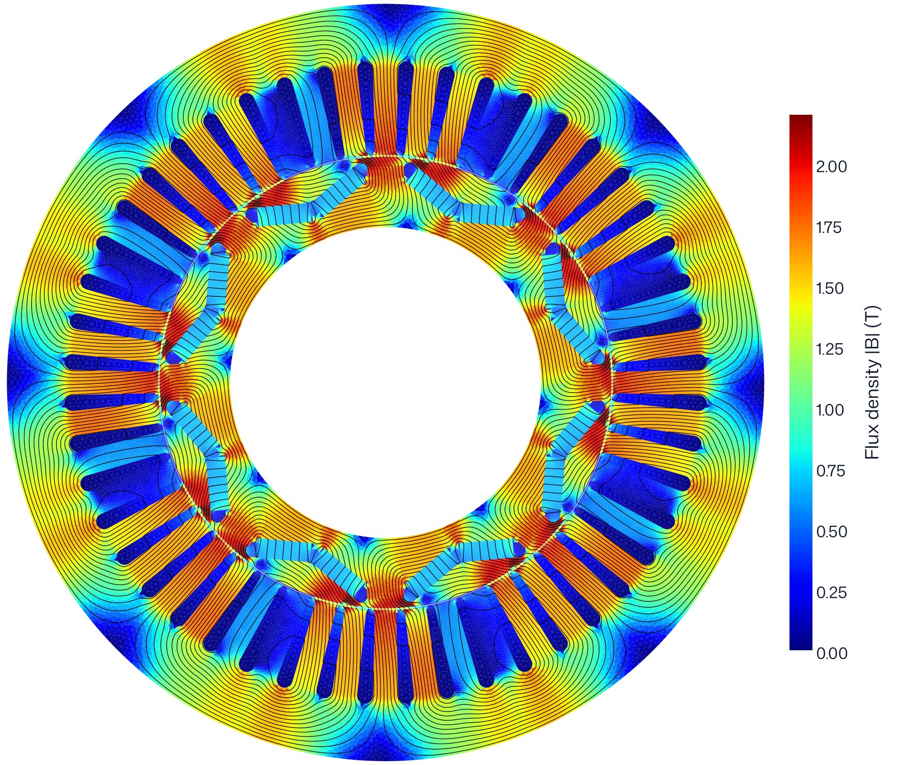
The model is a two-dimensional nonlinear magnetostatic finite element model, built and solved end to end in ElectroLeap: geometry, winding, mesh, field, torque, flux linkage, losses and maps. It covers one pole, one eighth of the machine, with anti-periodic boundaries, and the results are scaled to the full machine.
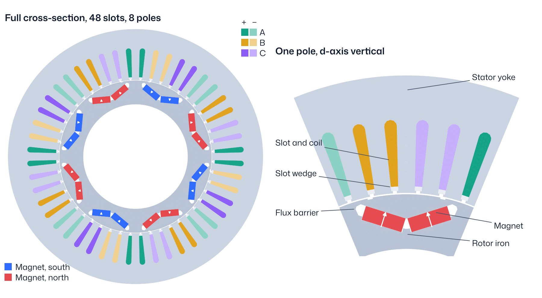
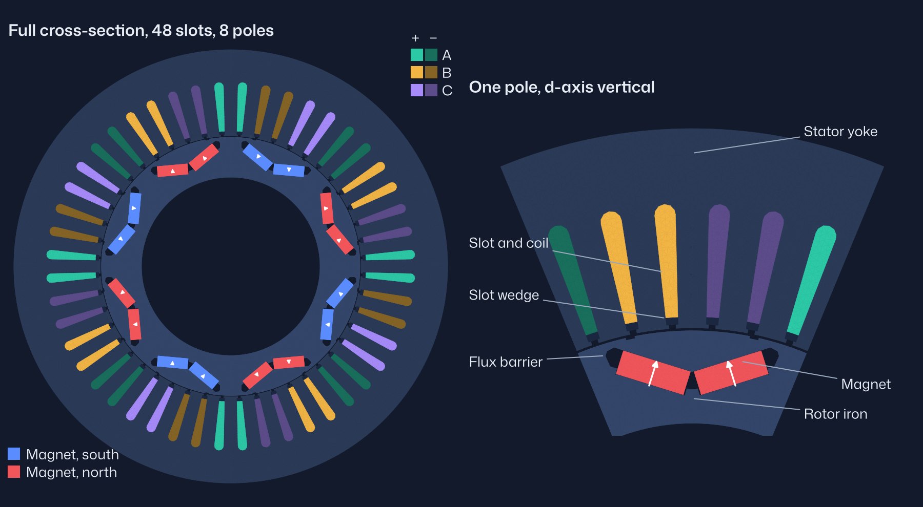
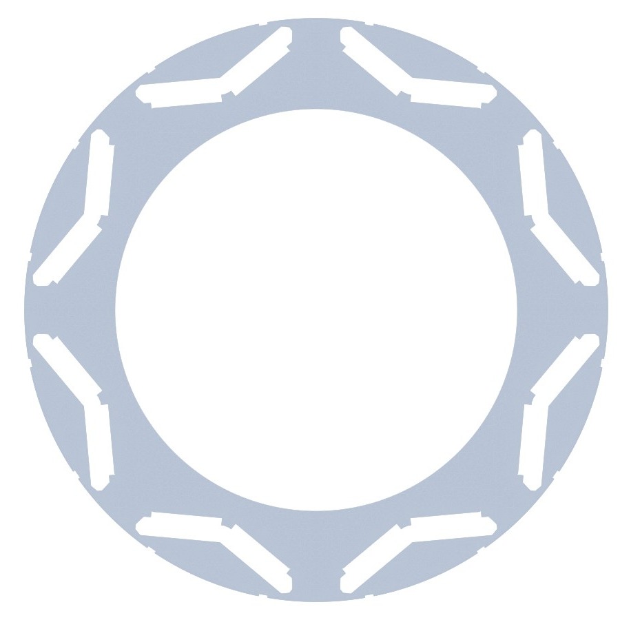
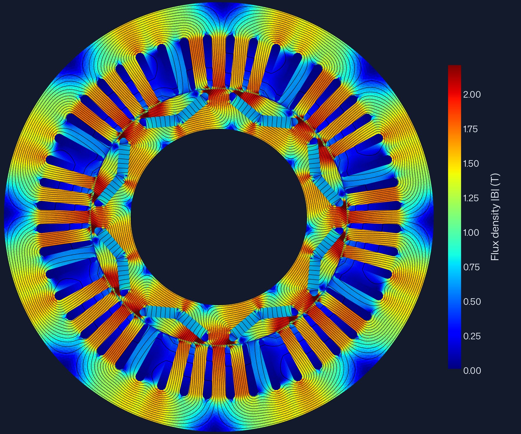
Table 2 lists the dimensions used in the model and where each comes from. The stator and rotor come from the dimensioned lamination drawing in [4]; the slot widths were fitted to the drawing outline. The magnet pocket was extracted from the vector paths of the same drawing and overlaid on all eight poles; the model outline is within 0.27 mm of it at worst and 0.08 mm on average. Figure 2 shows the model's rotor lamination. Rotor notches 0.6 mm deep at ±12° from the d-axis were added, since the drawing does not dimension them.
| Item | Value | Source |
|---|---|---|
| Stator outside diameter | 269.24 mm | [4] |
| Stator bore | 161.93 mm | [4] |
| Slots | 48 | [1] |
| Slot depth, opening | 33.53 mm, 1.93 mm | [4] |
| Tooth tip height, slot width below the tip | 1.02 mm, 3.15 mm | [4] |
| Slot bottom | round, Ø 5.64 mm | [4] |
| Tooth width near the bore | 7.62 mm | [4] |
| Air gap | 0.73 mm | [1] |
| Rotor outside diameter | 160.47 mm (drawing: 160.38 mm) | [1], [4] |
| Rotor inside diameter | 110.64 mm | [4] |
| Stack length, stacking factor | 83.6 mm, 0.97 | [1] |
| Lamination thickness | 0.33 mm, grade not published | [1] |
| Poles | 8 | [1] |
| Magnets | 16, two per pole in a V, 18.9 × 6.5 × 83.1 mm, sintered NdFeB | [1], [2] |
| V included angle | 145.3° | [4] |
| Outer bridge, minimum width | 1.43 mm | [4] |
| Turns per phase | 72: 9 per coil, 8 coils in series, one path | [1] |
| Phase resistance | 0.069 Ω at 21 °C | [1] |
| Ratings | 50 kW, 400 N·m, 6000 rpm, 500 V dc | [5] |
The air gap is 0.73 mm in the design table [1], while the two diameters on the drawing give 0.775 mm. The model uses the design table. With the drawing's gap the back-EMF is 1.0 % lower and the peak torque 0.7–1.0 % lower.

- Materials: the lamination grade is not published; the model uses M270-35A with its nonlinear B–H curve. Magnets: sintered NdFeB, parallel magnetisation, relative permeability 1.05, temperature coefficient −0.11 %/K, remanence as calibrated in §4.
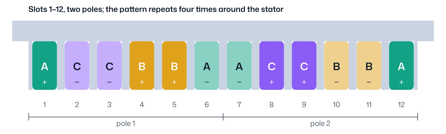
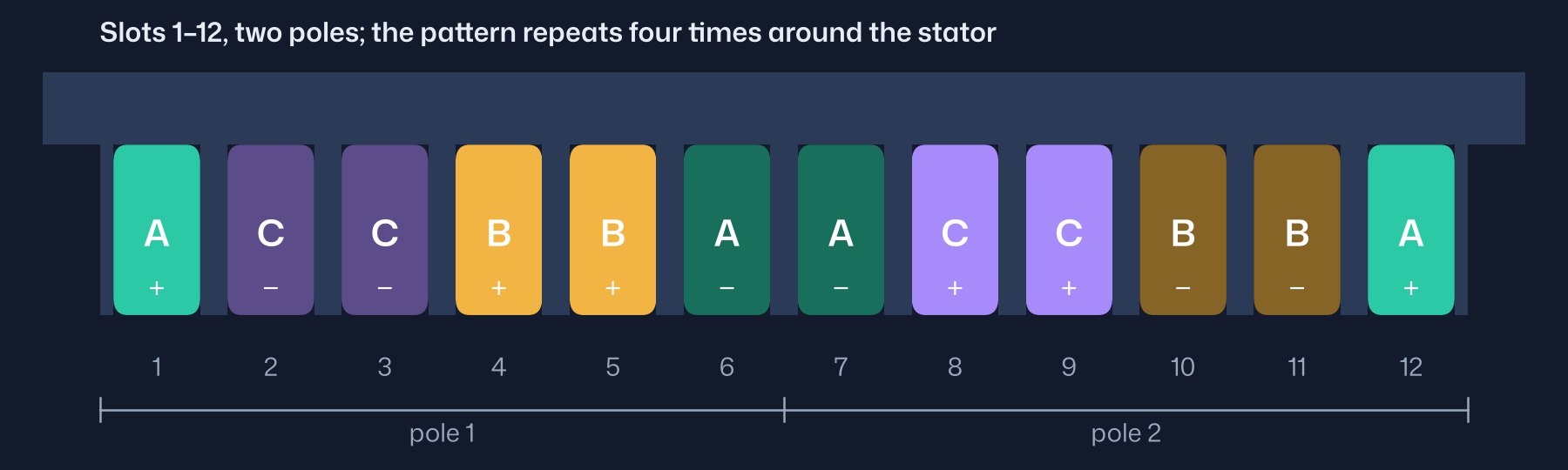
- Winding: three-phase, single layer, two slots per pole per phase, coil span 5 slots, fundamental winding factor 0.966. 9 turns per coil, 8 coils in series per phase, one parallel path, star connection, 72 turns per phase. Phase resistance 0.069 Ω at 21 °C. In two dimensions only the slot pattern matters, and it is the same for a coil span of 5, 6 or 7 slots.
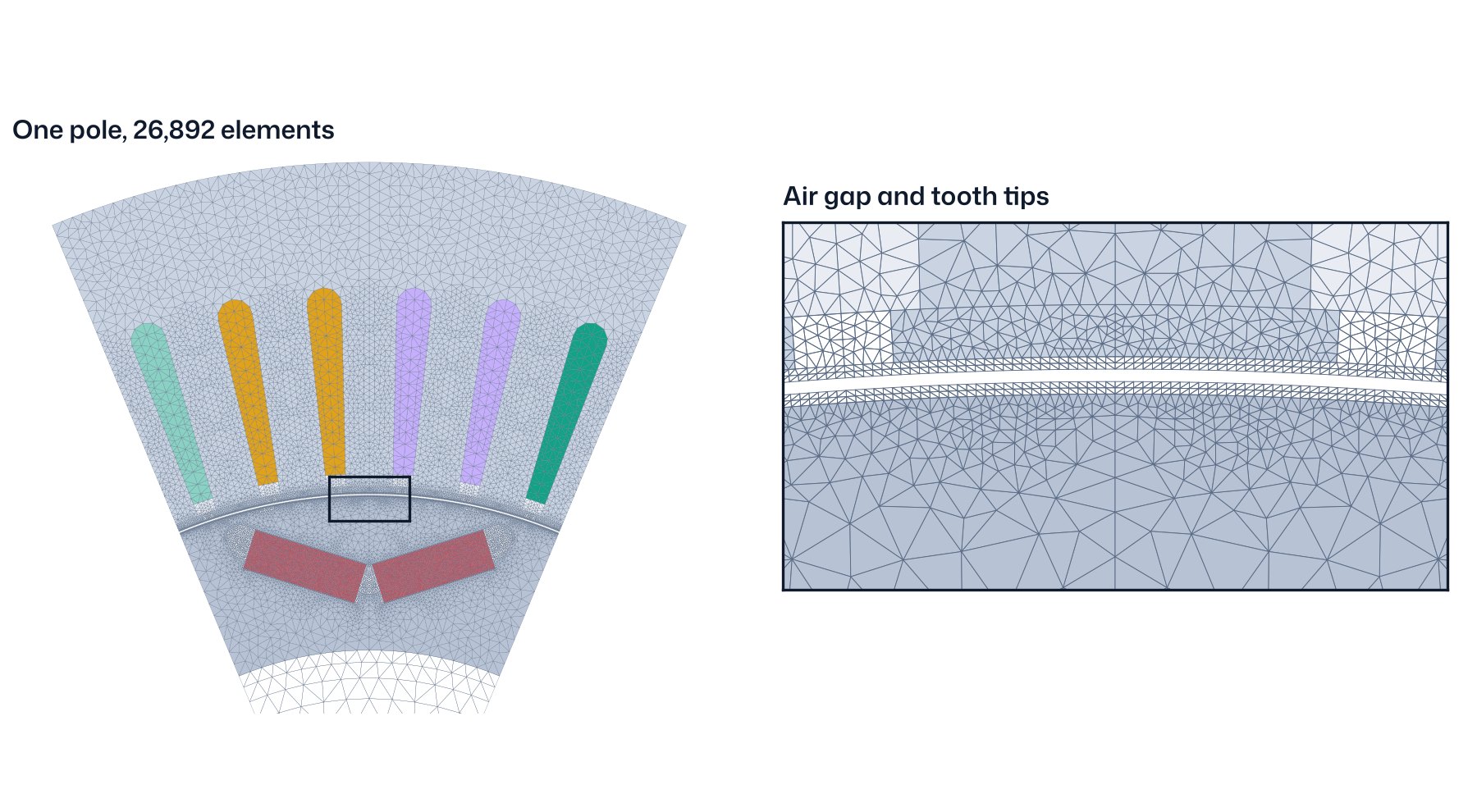
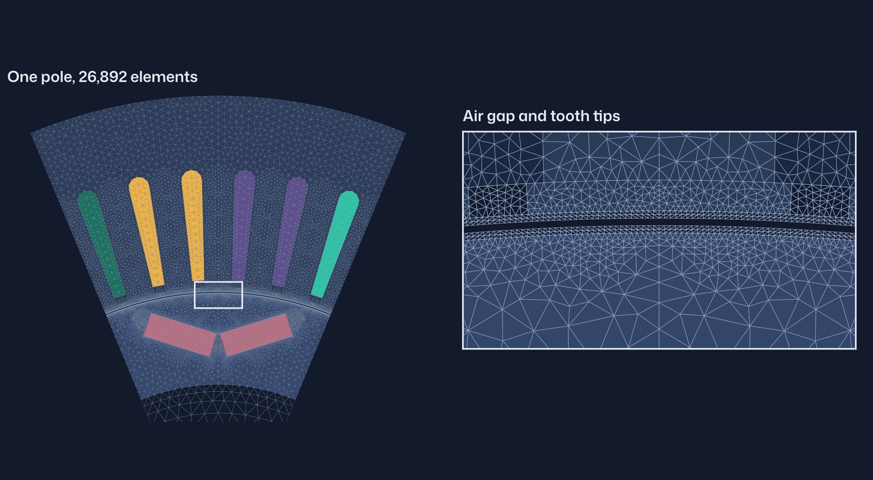
Each rotor position is one nonlinear field solve. Torque is computed from the air-gap field and flux linkage from the winding. Voltage, current, power factor, loss and efficiency follow from those through the same post-processing a user gets. Mesh convergence is in §15.
04What was calibrated
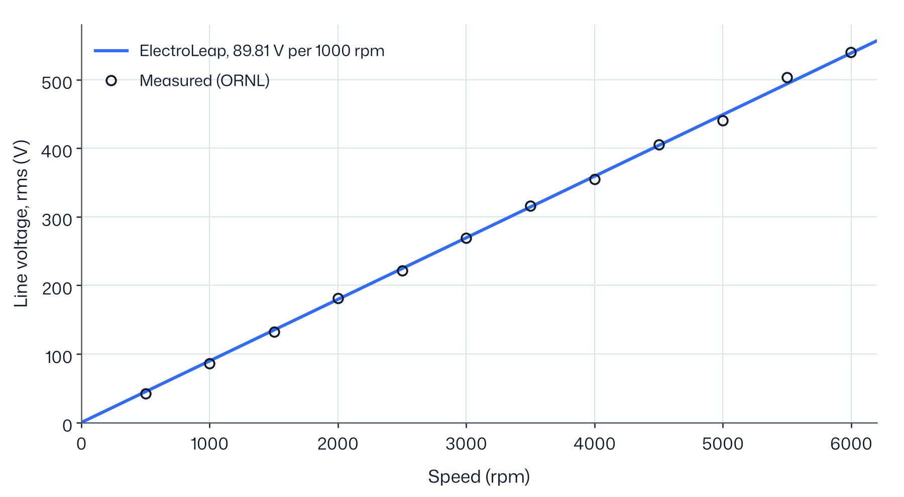
Magnet remanence. With the published magnet data, 1.255 T at 20 °C, the model's back-EMF constant is 105.30 V/krpm, 17.3 % above the measured 89.78 V/krpm. Torque and current scale with the magnet flux, so a model that is 17 % strong at no load cannot be used for the other comparisons. We set the remanence so that the back-EMF matches: 1.101 T at 20 °C, 12.3 % below the published value. We checked four explanations against the reports:
- Magnet temperature: ruled out. A 12 % drop would need the magnets at about 130 °C in a test with oil at 25 °C, and the back-EMF constant does not change with speed.
- Incomplete magnetisation: possible. The magnets are magnetised after assembly in the rotor, and a pulse that does not saturate every part of the magnet leaves a lower remanence than the sample on which the material data were measured.
- Three-dimensional end leakage: possible. Flux that closes at the stack ends, outside the winding, lowers the back-EMF without changing the field in the middle of the stack. The air-gap probe cannot settle it: its position is not stated, and the calibrated two-dimensional model already reproduces its reading at the tooth centre (§6).
- The magnet data: the other published magnet line, 1.24 T with a relative permeability of 1.12, lowers the back-EMF by only 1.8 %.
The measurements cannot separate magnetisation from end leakage. The calibrated remanence holds their sum and is an effective value for this rotor, not a material property.
Iron-loss build factor. The second calibration came after the first loss results (§10): one factor of 1.410 that multiplies every iron loss, fitted by least squares on the measured no-load loss from 1500 to 6000 rpm. It was not refitted on the voltage sweep or on the efficiency map. Results are shown both without it and with it.
Nothing was fitted on the torque, the currents or the efficiency. One angle offset places the model on the measured shaft angle, which has an arbitrary origin (§7).
05Back-EMF and waveform
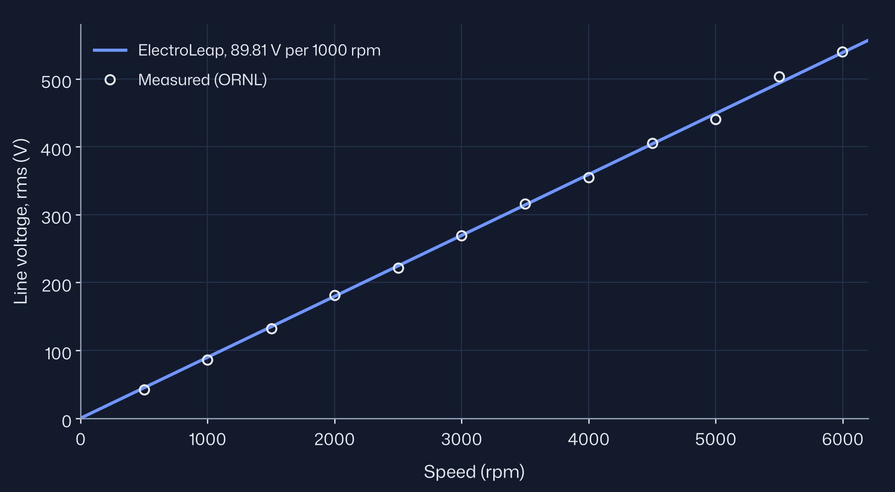
The line-to-line back-EMF is computed from the phase flux linkage over one electrical period at 192 rotor positions, at 25 °C. The constant is the calibration target, so the agreement of the slope is by construction. The per-speed points are a check on linearity: the largest differences are −9.5 V at 5500 rpm and +8.6 V at 5000 rpm, about 2 %. They are adjacent points of opposite sign, which points to scatter in the readings rather than to the model. The two lowest speeds read 7 % and 5 % low on the measurement.
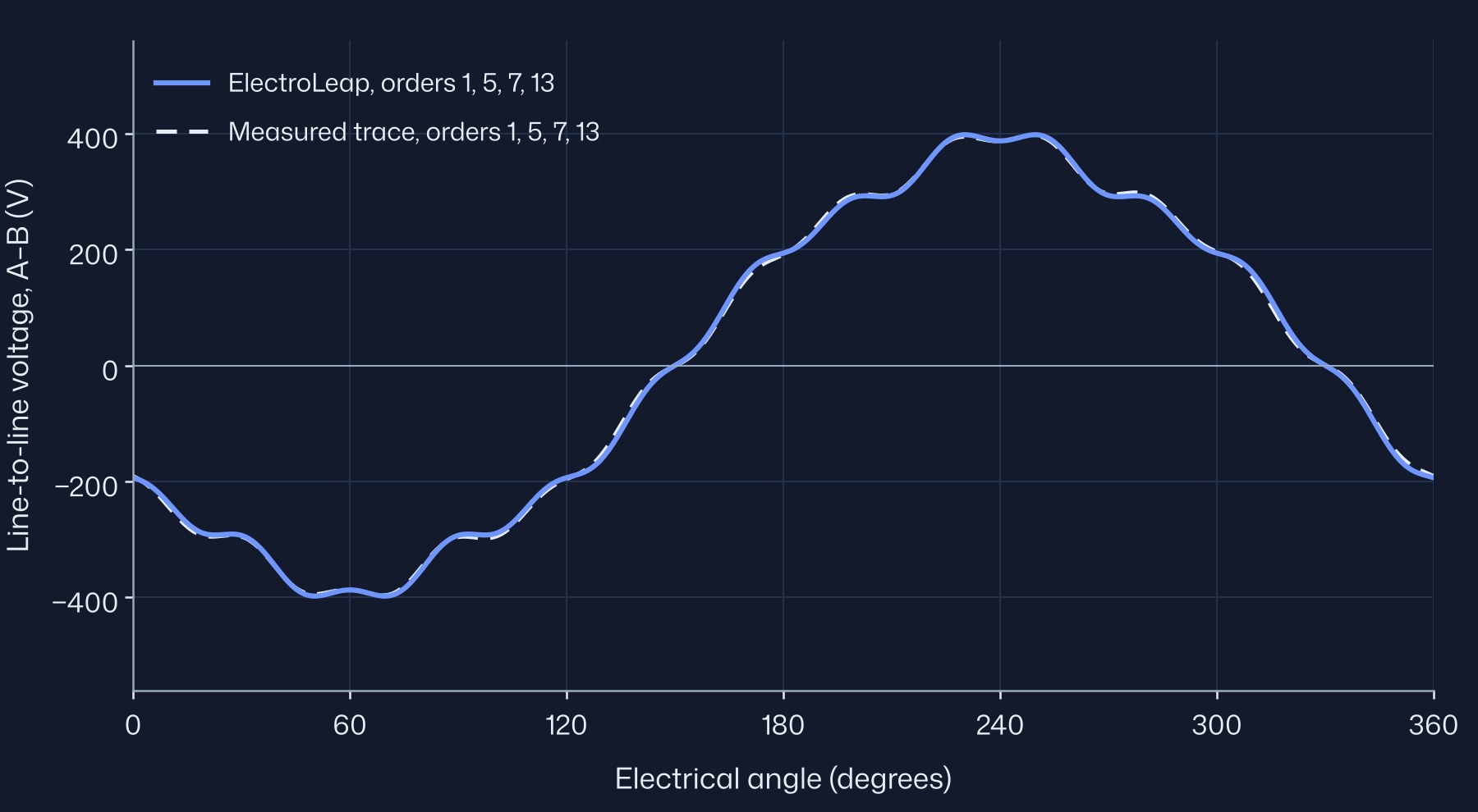
The waveform is a prediction. Figure 7 shows the model's line-to-line voltage at the two speeds where ORNL recorded oscilloscope traces. The ripple on the waveform comes from the slots: as the rotor passes each tooth, the flux through the coils changes in small steps, at the slot harmonics of order 12k ± 1 (11 and 13, 23 and 25, and so on).
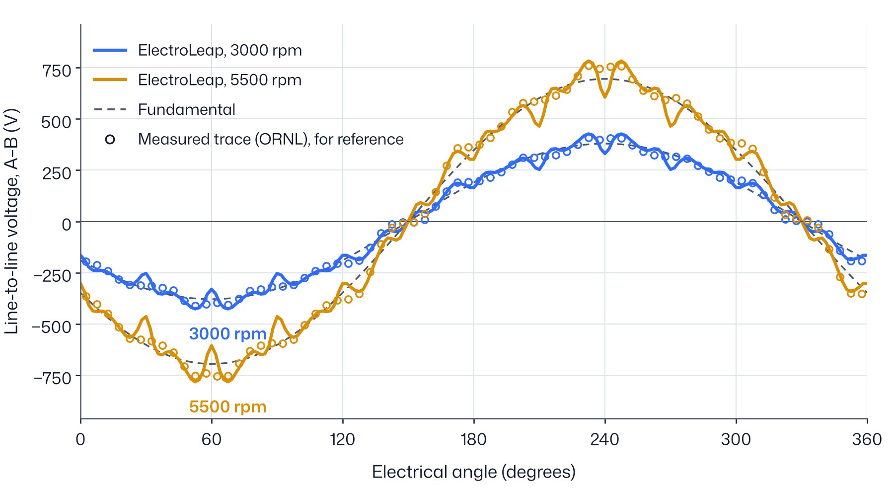
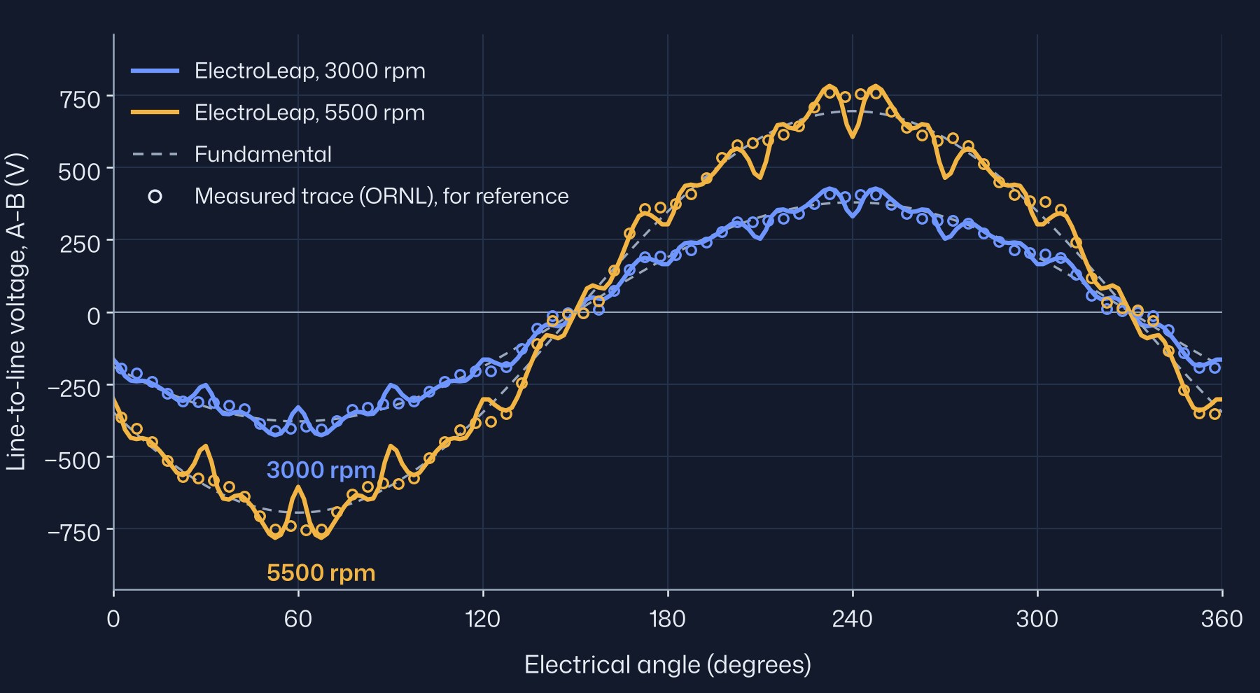
The published traces have no voltage scale. To overlay them, each trace was digitised from the report, scaled to the rms voltage ORNL measured at that speed (269.3 V and 503.4 V) and shifted in time so that its fundamental lines up with the model's. Nothing in the trace is scaled to the model. The fundamentals then agree within 0.1 % at 3000 rpm and 2.1 % at 5500 rpm, and ORNL's own peak readings, to the nearest 25 V, are 425 V and 775 V against 427 V and 783 V in the model. The shape is compared through the harmonics, as a percentage of the fundamental, and through the peak-to-rms ratio. In two dimensions those percentages do not depend on speed, so the model values are the same at both speeds.
| Measured, 3000 rpm | ElectroLeap, 3000 rpm | Measured, 5500 rpm | ElectroLeap, 5500 rpm | |
|---|---|---|---|---|
| 5th harmonic, % of fundamental | 3.4 | 4.68 | 3.4 | 4.68 |
| 7th | 2.6 | 1.74 | 2.4 | 1.74 |
| 11th | 5.8 | 1.03 | 5.3 | 1.03 |
| 13th | 4.2 | 4.34 | 3.8 | 4.34 |
| Peak / rms | 1.515 | 1.585 | 1.531 | 1.585 |
| Peak voltage (V) | 425 | 427 | 775 | 783 |
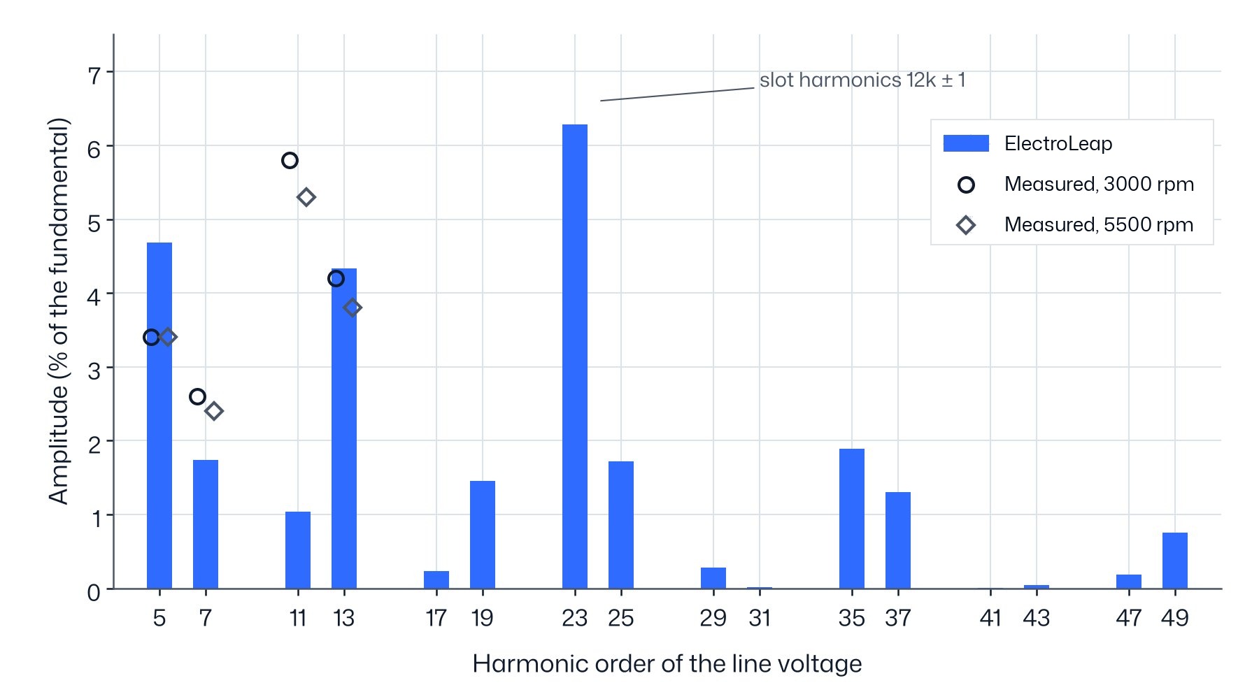
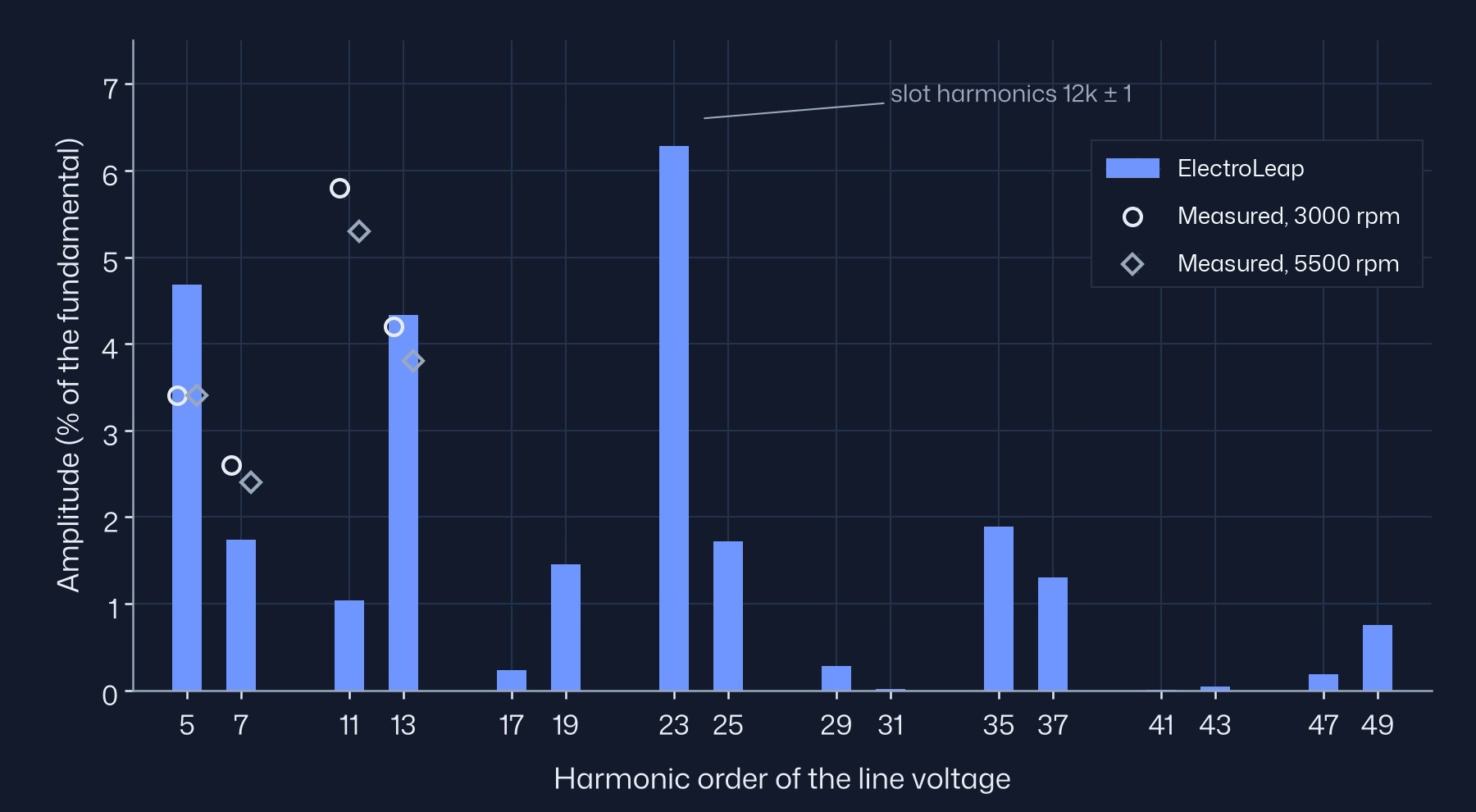
The model's total harmonic distortion is 9.8 % of the fundamental. The largest harmonic is the 23rd, 6.3 %, and it comes from the rotor notches: without them the 23rd falls to 0.7 %. The notch shape is not published and had to be assumed (§3), so the 23rd, like the 11th below, reflects that assumption. The digitised traces resolve orders up to the 13th only, so the 23rd cannot be checked against the measurement.
The model's 5th, 7th and 13th differ from the measurement by at most 1.3 % of the fundamental. The 11th is 4–5 % of the fundamental low, outside the digitising uncertainty. The traces also give the phase of each harmonic: the 5th, 7th and 13th have the same phase in the model and in the measurement, but the model's 11th is in opposite phase. The rotor notches explain this. Without them the model's 11th is 8.5 %, in phase with the measurement, and the 13th falls to 0.8 %. The assumed notches take about 9.5 % off the 11th and turn it over, while the real rotor takes off about 3 %: for the 11th, the assumed notch is about three times too strong. The notch shape is not dimensioned in the published drawing. A notch 0.4 mm deep centred at 11°, instead of 0.6 mm at 12°, brings the 11th to 5.5 %, inside the measured range, but we did not adopt it: choosing a notch to match a harmonic would be a third calibration.
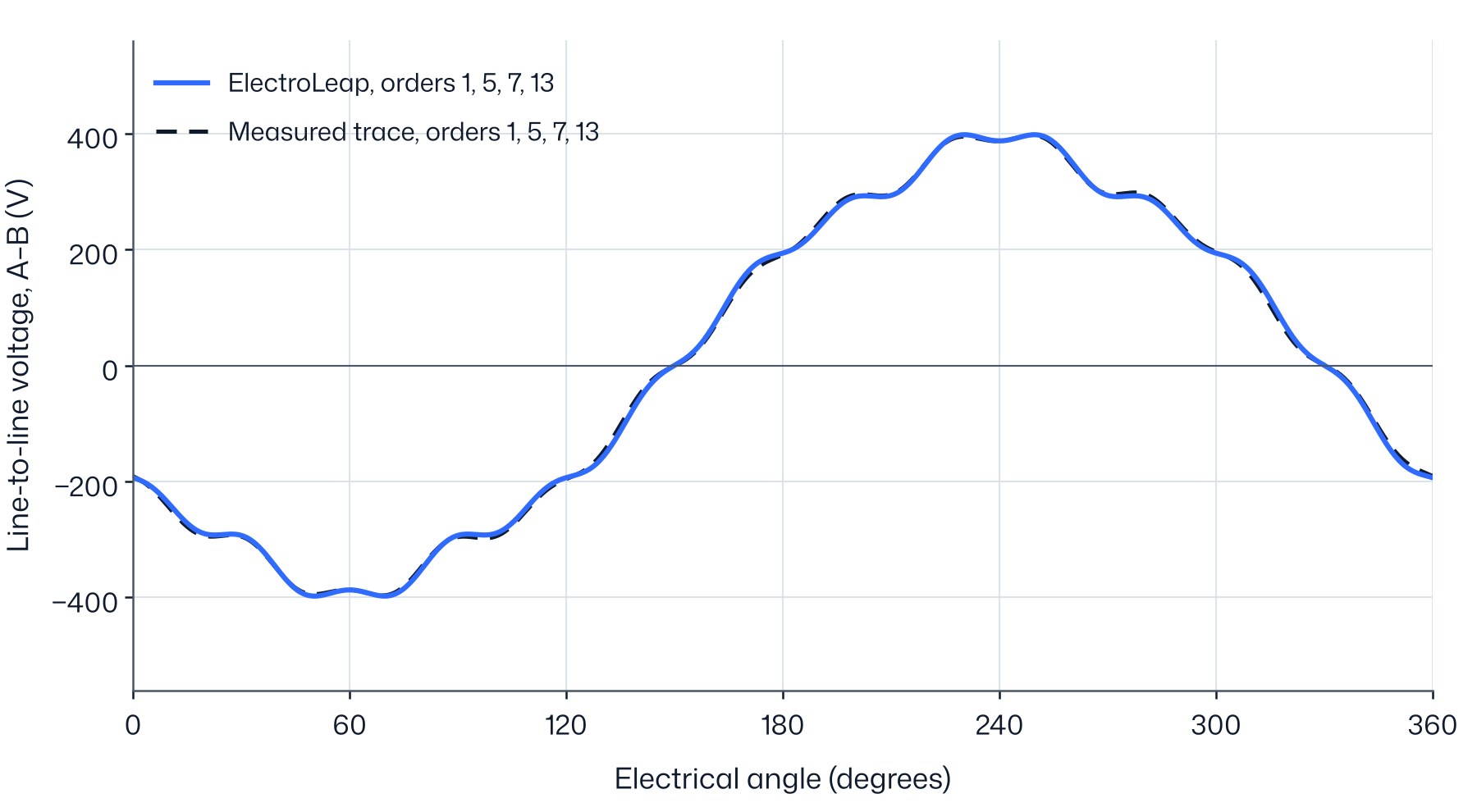
Figure 9 compares the two waveforms with the 11th and the orders above the 13th left out: the 11th because it depends on the notch shape, which is not published, and the orders above the 13th because the digitised traces cannot resolve them. The two then agree within 1.7 % rms of the fundamental at 3000 rpm and 2.8 % at 5500 rpm, against 8.3 % for the full waveforms.
06Air-gap flux density
ORNL measured the no-load air-gap flux density at one point per slot over two poles. The probe radius, its axial position and whether each reading sits over a tooth or a slot opening are not stated. The model is sampled in the middle of the air gap, at the centre of each tooth.
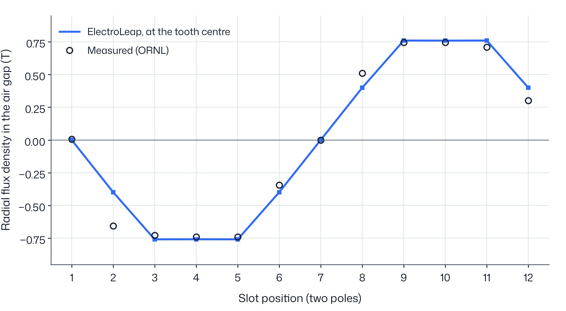
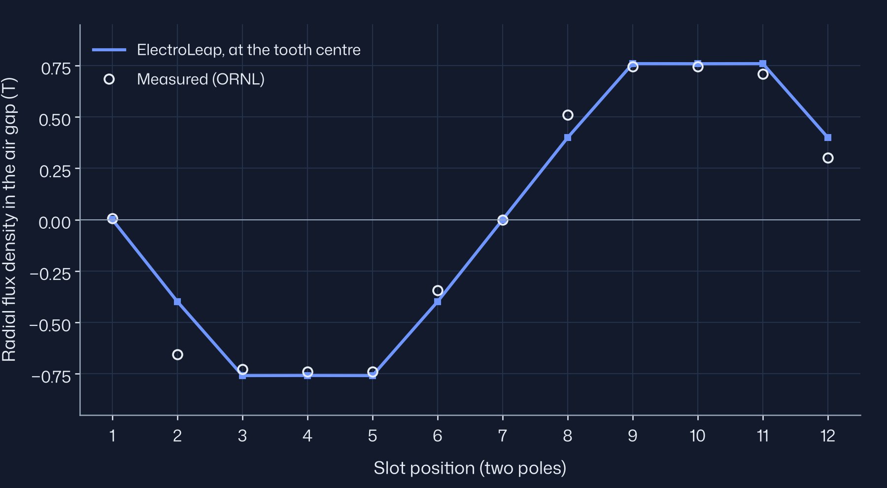
The fundamental of the model matches the measured 0.824 T and the peak is 1.8 % above it. The largest local differences are at slots 2, 8 and 12, on the flanks of the wave, where the field changes fastest from one slot to the next and a small offset in probe position moves the reading most. The probe origin is not stated, so the measured points are placed by slot index.
07Locked-rotor torque
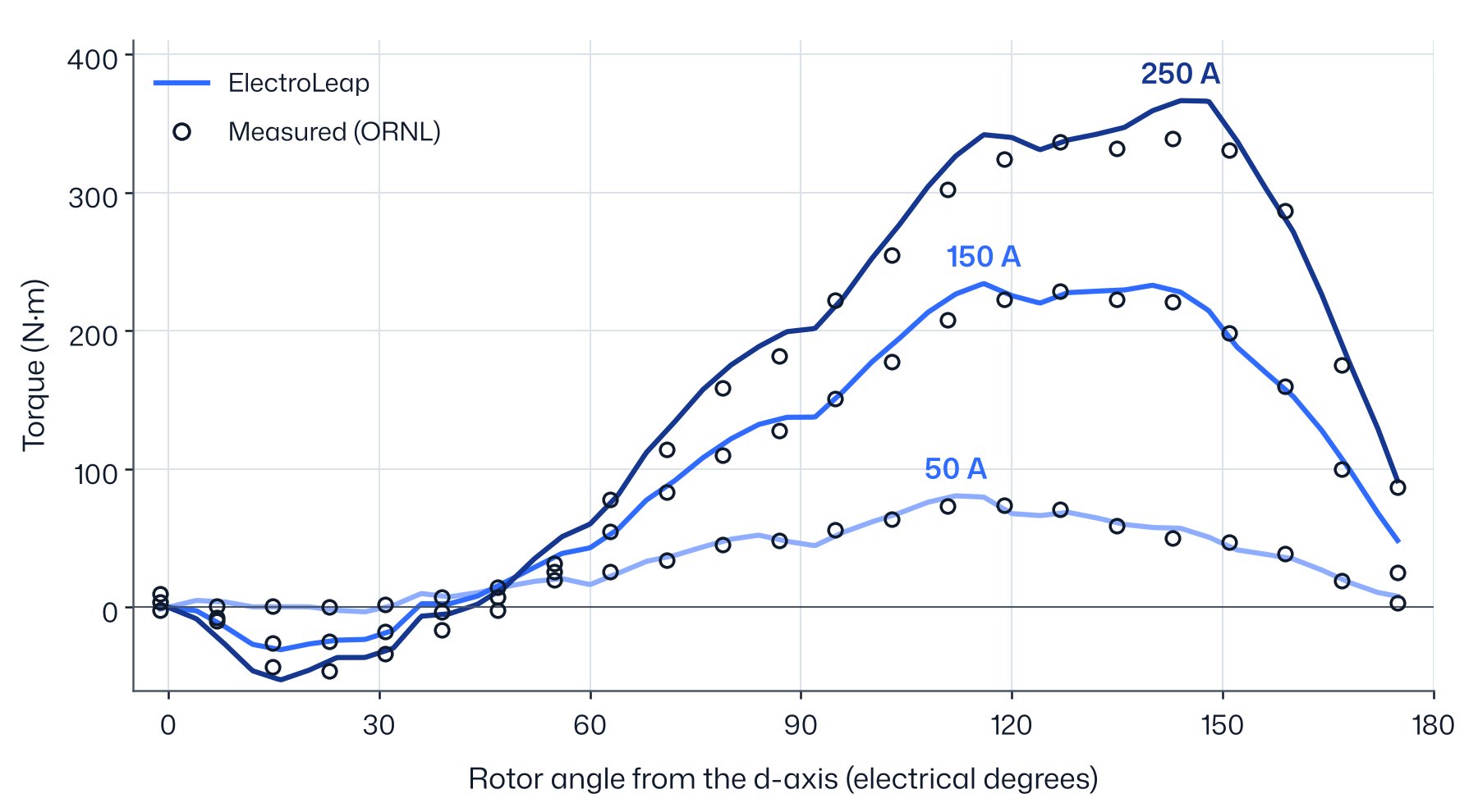
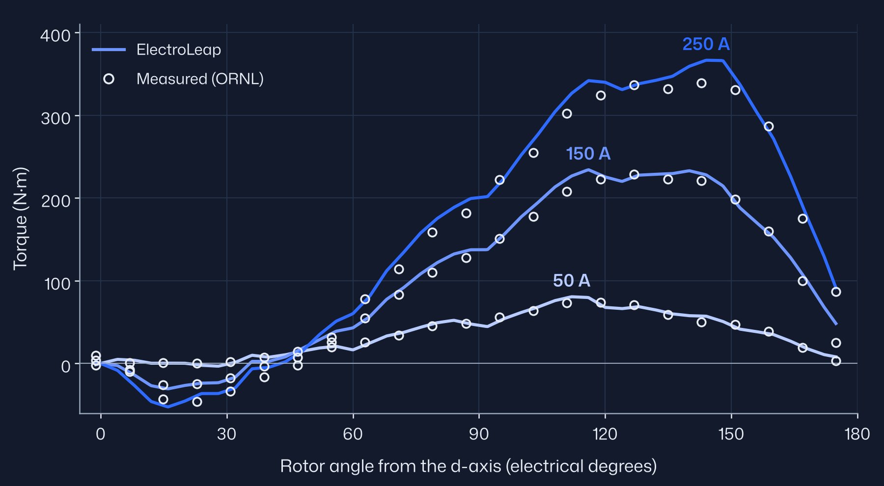
The rotor is held at a series of angles while dc currents (I, −I/2, −I/2) flow in the three phases, and the torque is measured at each angle. The test sweeps the full torque curve at a fixed current vector, so the magnet torque and the reluctance torque both appear. The model runs the same test: the product's locked-rotor run, 0–90° mechanical in 1° steps.
The measured shaft angle has an arbitrary origin, and it runs in the opposite direction to the model angle, as the test report describes. One offset places the model on it. It was fitted on the 50 A curve only and then frozen for every other current. Before the runs we set acceptance levels for the peak torque, 5 % from 50 to 150 A and 8 % at 200 and 250 A, and for the rms difference over the curve, 8 % of the measured peak. The peaks below compare the model at the same 23 angles as the measurement; the model's full 1° sweep peaks slightly higher, at 234.3 N·m for 150 A.
| Current (A) | Measured (N·m) | ElectroLeap (N·m) | Peak difference | Curve rms |
|---|---|---|---|---|
| 50 | 74.0 | 79.30 | +7.16 % | 4.18 % |
| 75 | 117.7 | 121.08 | +2.87 % | 3.97 % |
| 100 | 158.0 | 157.42 | −0.37 % | 2.99 % |
| 125 | 199.0 | 193.47 | −2.78 % | 3.10 % |
| 150 | 229.0 | 229.46 | +0.20 % | 3.54 % |
| 200 | 286.6 | 304.89 | +6.38 % | 3.94 % |
| 250 | 339.0 | 364.49 | +7.52 % | 3.67 % |
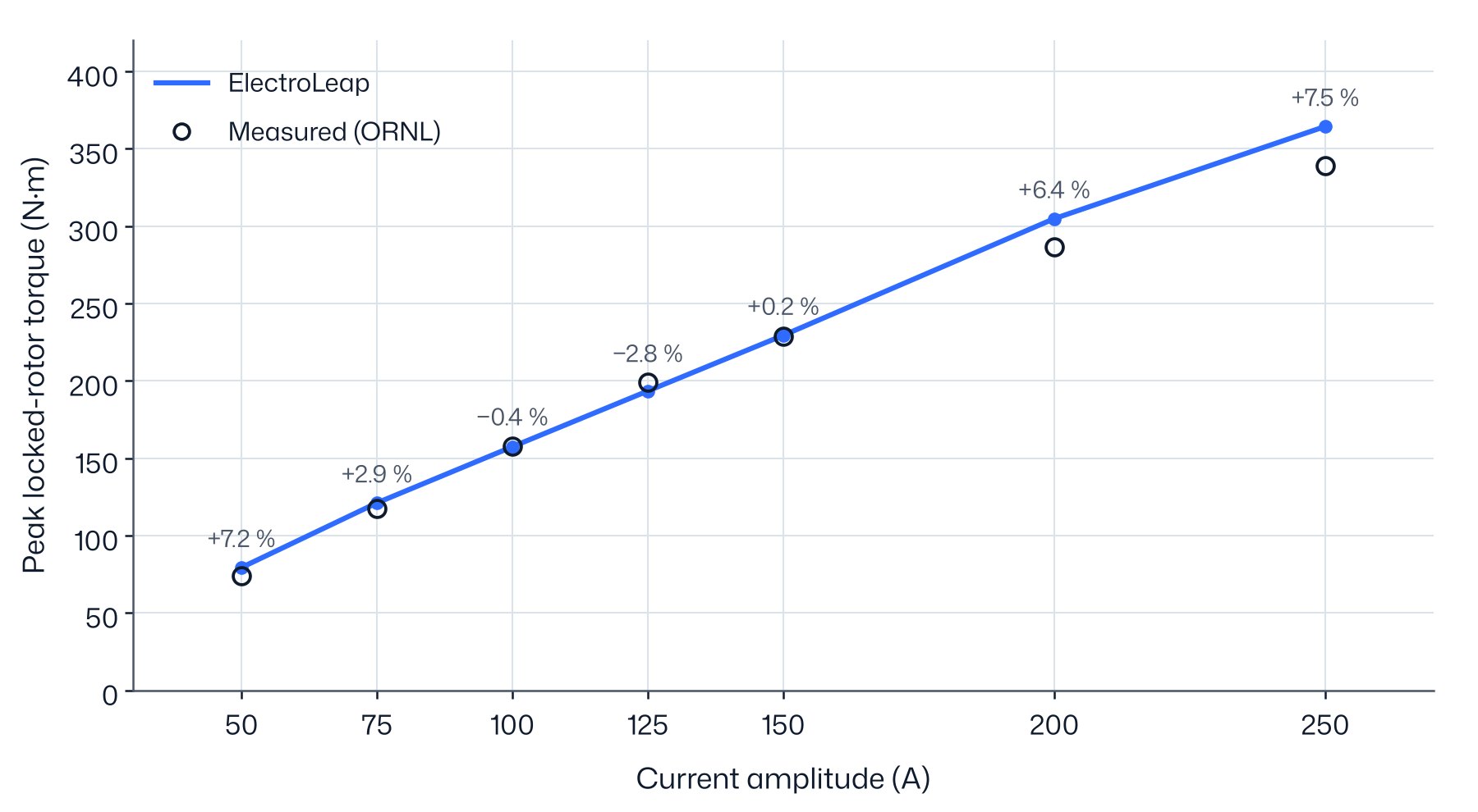
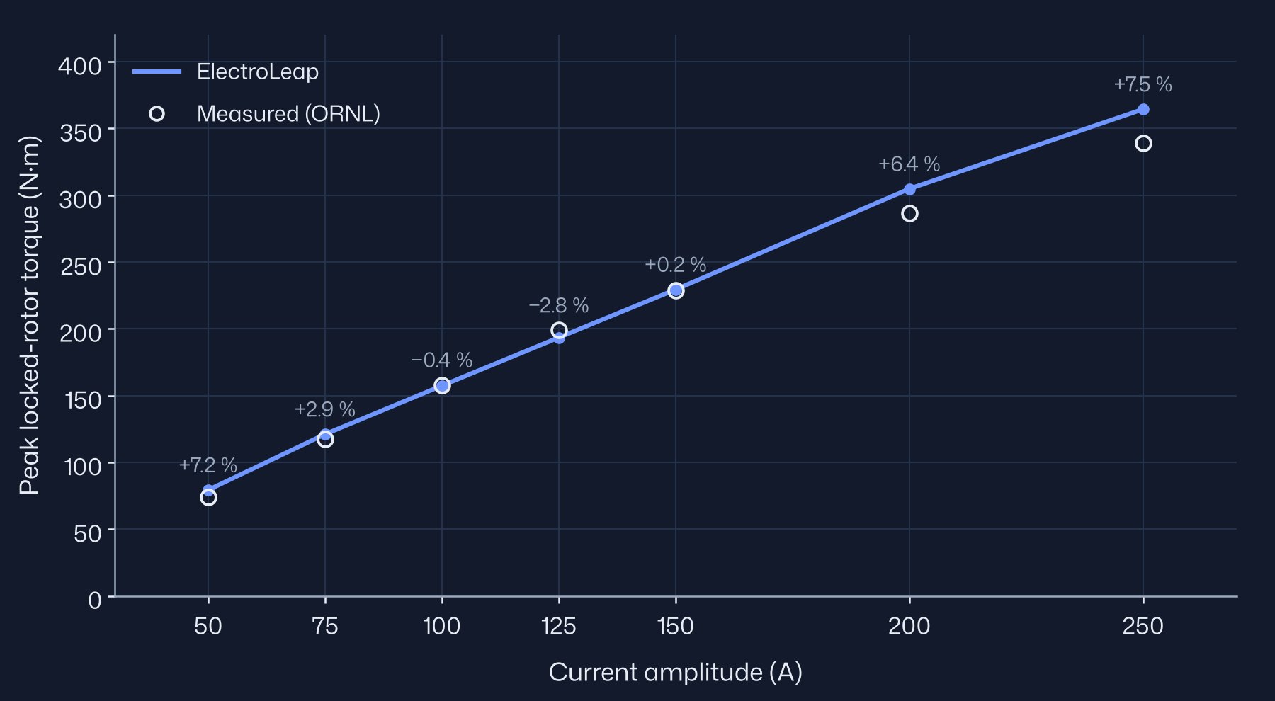
Six of the seven peaks are inside their level, and every curve is inside 8 % rms. The 50 A peak is 7.2 % high and misses its 5 % level. The 50 A peak is sensitive to that offset: moving it by 1° changes it to +8.1 % and takes the 75 A and 250 A peaks across their levels as well. The assumed notch shape (§5) is the other sensitive input: in our sensitivity runs it moved the 50 A peak by up to 3.7 %, more than at any other current. At 200 and 250 A the model reads 6–8 % high, inside the 8 % level but with a clear trend. The cause is not identified from this data; the unpublished lamination grade is one candidate.
08Load points at 900 rpm
At 900 rpm ORNL ran the motor on a 60 Hz sinusoidal supply without an inverter, with the voltage chosen for the best efficiency at each torque. Sinusoidal currents are what the model assumes, so these are the cleanest load comparisons in the data. For each measured torque and voltage the model finds the current and current angle that give that torque at that voltage, then reports the current and the power factor. The winding resistance is taken at the measured temperature: the oil temperature on the light-load rows, and a band 20 to 40 °C below the winding hot-spot reading on the peak rows.
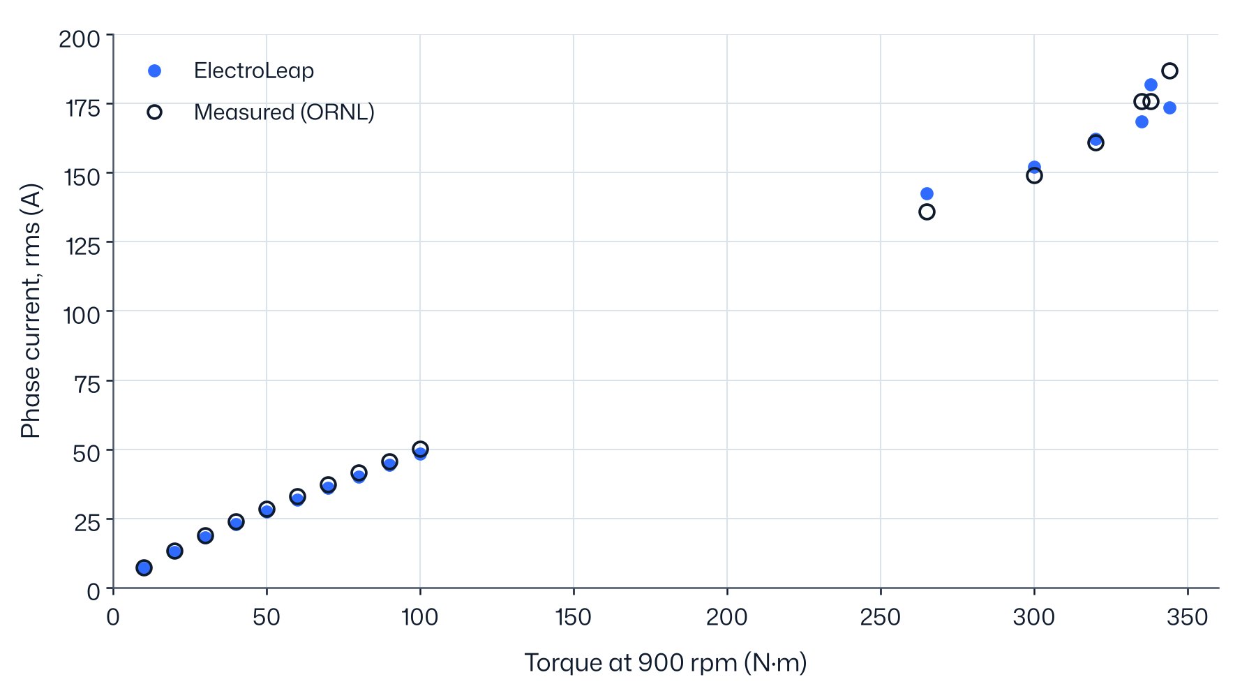
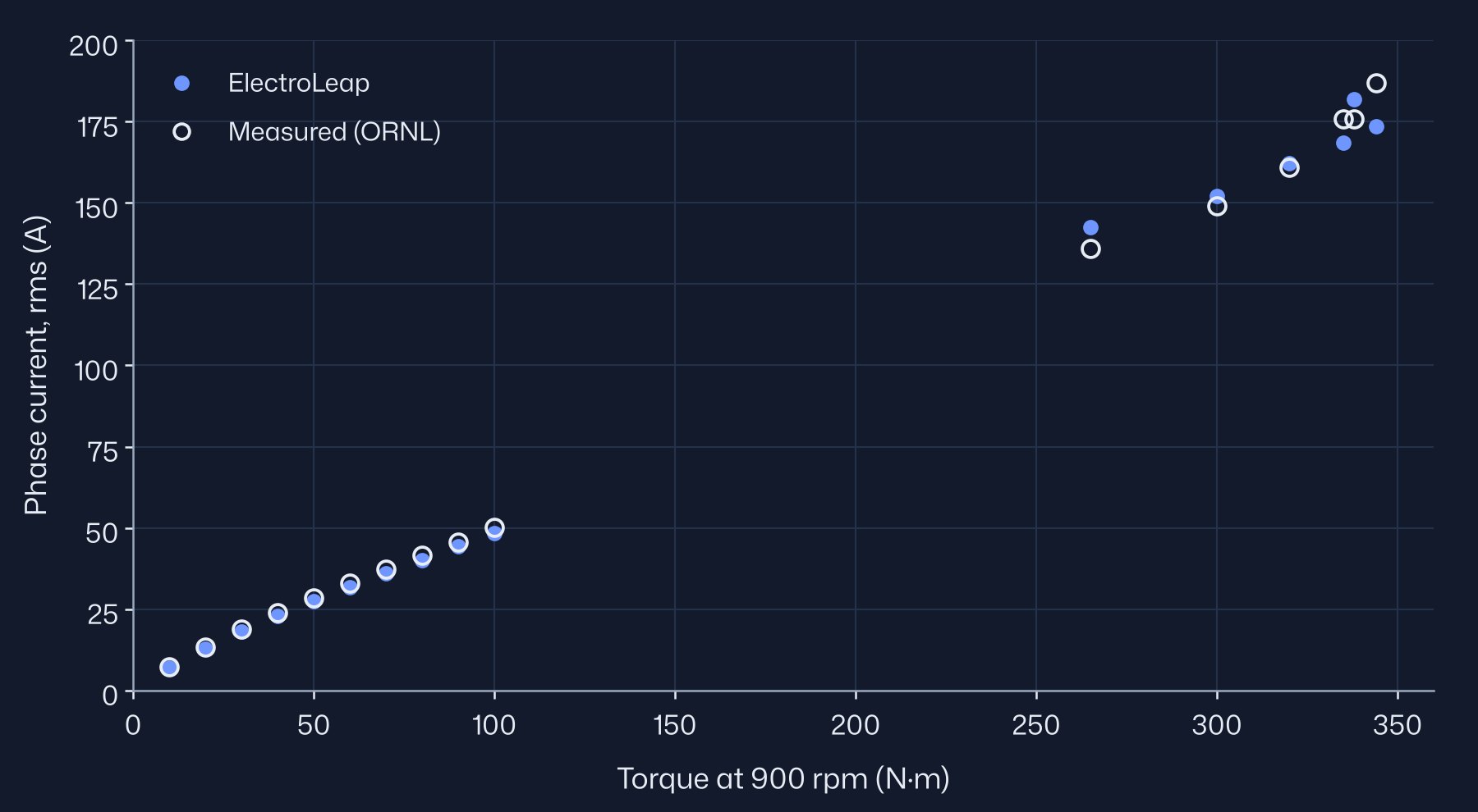
| Torque (N·m) | Line voltage (V) | Measured (A) | ElectroLeap (A) | Difference | Power factor, measured | Power factor, ElectroLeap |
|---|---|---|---|---|---|---|
| 20 | 90 | 13.3 | 12.68 | −4.7 % | 0.98 | 0.97 |
| 50 | 115 | 28.5 | 27.38 | −3.9 % | 0.89 | 0.89 |
| 100 | 140 | 50.1 | 48.40 | −3.4 % | 0.84 | 0.85 |
| 265 | 205 | 136 | 142.53 | +4.8 % | ||
| 300 | 205 | 149 | 152.08 | +2.1 % | ||
| 320 | 205 | 161 | 162.13 | +0.7 % | ||
| 335 | 205 | 176 | 168.58 | −4.2 % | ||
| 344 | 205 | 187 | 173.49 | −7.2 % |
From 20 to 100 N·m the model current is 3–5 % below the measurement and the power factor is within about 0.02. The model has no end-winding leakage, one candidate for this offset. At 10 N·m the current is 6.85 A against 7.3 A. On the peak rows the difference changes sign with torque, from +4.8 % to −7.2 %. Those rows were taken at changing winding temperatures, and no oil or magnet temperature is published for them, so the magnets stay at 25 °C in the model; hotter magnets would raise the model current. The power factors published for the peak rows imply about 23 kW of loss at 25 kW of output and are not compared. A 338 N·m row at 210 V has no published temperature and is left out of the table.
09Voltage sweep at 900 rpm
In the same setup, with no load on the shaft, ORNL raised the supply voltage from 80 to 210 V and recorded the current. The open-circuit voltage at 900 rpm is about 81 V, so above it the current is almost pure d-axis current that strengthens the magnet field to hold the higher voltage. This test checks the d-axis and the saturation of the iron, and it does not depend on the loss model.
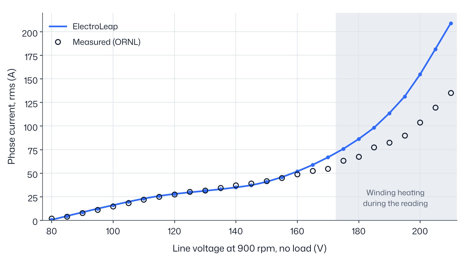
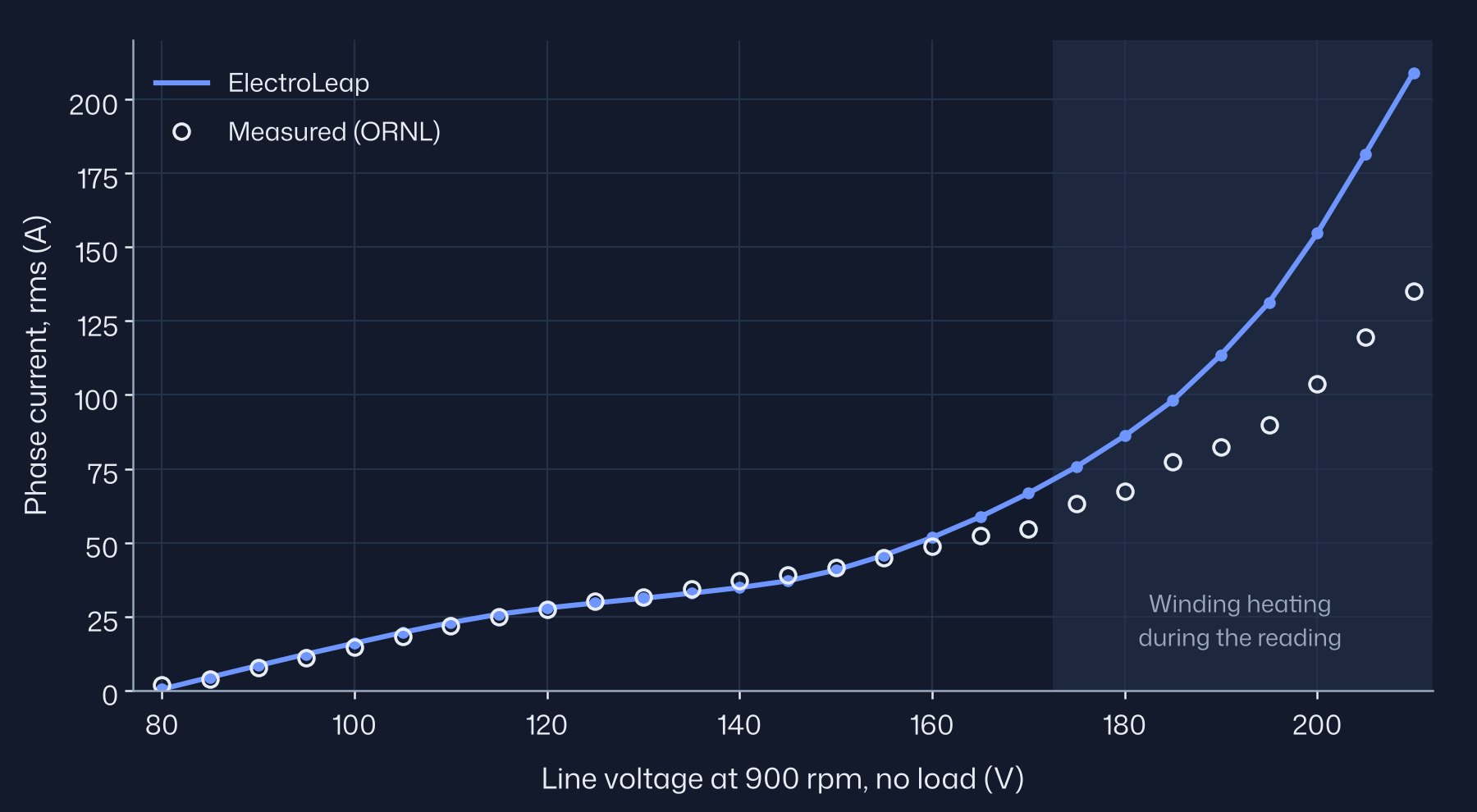
From 85 to 155 V the current is within about 2 A of the measurement. Above 155 V the model current grows faster than the measurement: +3 A at 160 V, +6 A at 165 V, +12 A at 170 V, and much more on the rows above 175 V, which were taken while the winding temperature was still rising. The growth is faster than linear, which points to a saturation mismatch between M270-35A and the unpublished Prius lamination: the model needs more current than the motor to push the flux higher. At 80 V the model gives only the field-setting current, 0.3 A, while the measured 1.9 A also carries the loss current.
The measured input power in this sweep rises by 720 W from 80 to 170 V. In the model that increase is almost all copper loss, 990 W, with the iron and magnet loss adding 76 W. The extra model current above 155 V shows up as extra copper loss, so the loss comparison follows the current comparison.
10No-load loss
ORNL measured the loss of the whole drive with the real rotor and again with a dummy rotor without laminations or magnets; the difference is the motor-rotor loss. With the stator open-circuit, that is the iron and magnet loss of the spinning field, plus any extra windage and oil drag of the real rotor over the dummy. The model has the first part only, so before running it we expected it to read low.
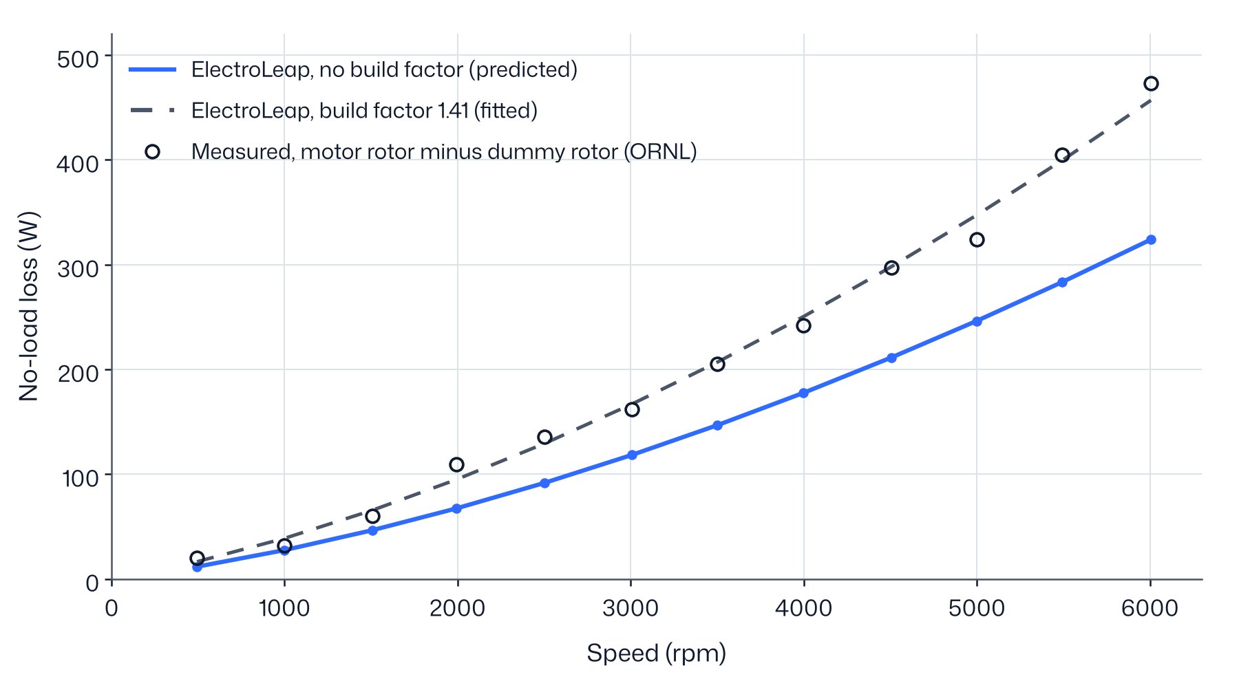
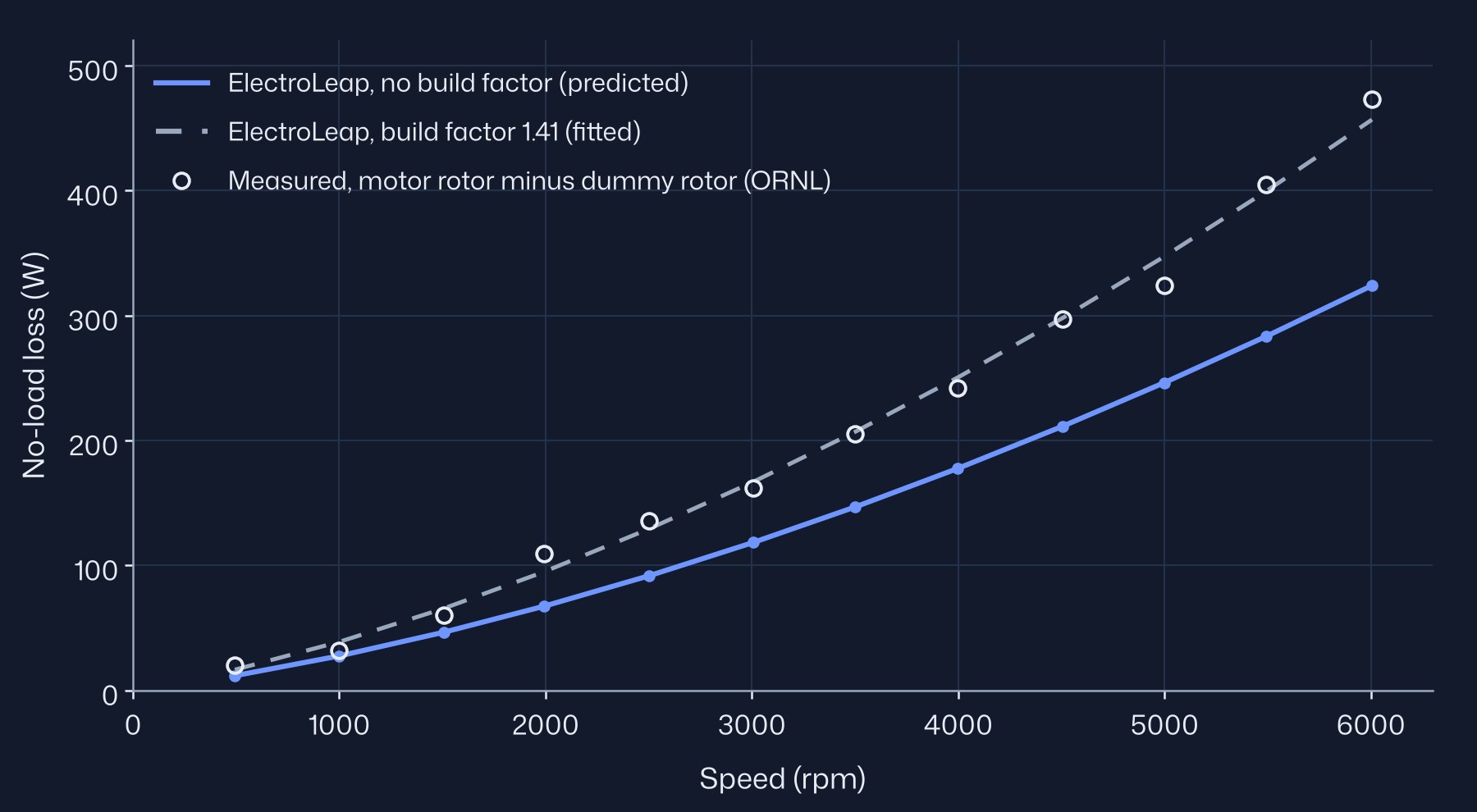
| Speed (rpm) | Measured (W) | Model, no factor (W) | Ratio | Model, factor 1.41 (W) |
|---|---|---|---|---|
| 1506 | 60.2 | 46.4 | 0.77 | 65.4 |
| 1991 | 109.0 | 67.1 | 0.62 | 94.7 |
| 3007 | 161.7 | 118.3 | 0.73 | 166.8 |
| 3999 | 242.1 | 177.6 | 0.73 | 250.4 |
| 4999 | 323.9 | 246.2 | 0.76 | 347.2 |
| 6006 | 472.8 | 323.9 | 0.69 | 456.8 |
Without a factor the model is low at every speed, by a ratio of 0.62 to 0.77 that does not trend with speed. The factor of 1.41 is the least-squares match on the ten points from 1500 rpm, so the dashed curve agrees by construction. The two points below 1500 rpm were not used; they read 3 W low and 7 W high with the factor. Of the 1.41, most compensates the lower lamination flux that comes with the calibrated remanence: fitted on the model with the published magnet data, the same factor would be 1.04. If the back-EMF gap is end leakage rather than magnetisation, the real lamination flux is nearer that model. The rest of the factor covers manufacturing effects on the steel and the extra drag of the real rotor, which this data cannot separate.
11Efficiency map
The measured map is the motor alone, inverter-fed at 500 V with pulse-width modulation (PWM), over-modulated at high speed, with the rotor coupled directly to the dynamometer. The windings reached about 200 °C in the high-torque tests, and per-point temperatures are not published. The model uses sinusoidal currents, winding at 100 °C, magnets at 80 °C, a current limit of 280.4 A and the same 500 V bus. Mechanical losses are set to zero. Before computing the map we expected it to read 1–2 % high.
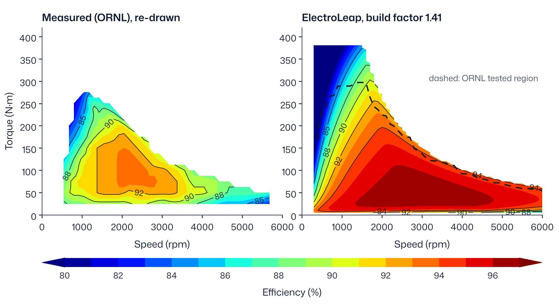
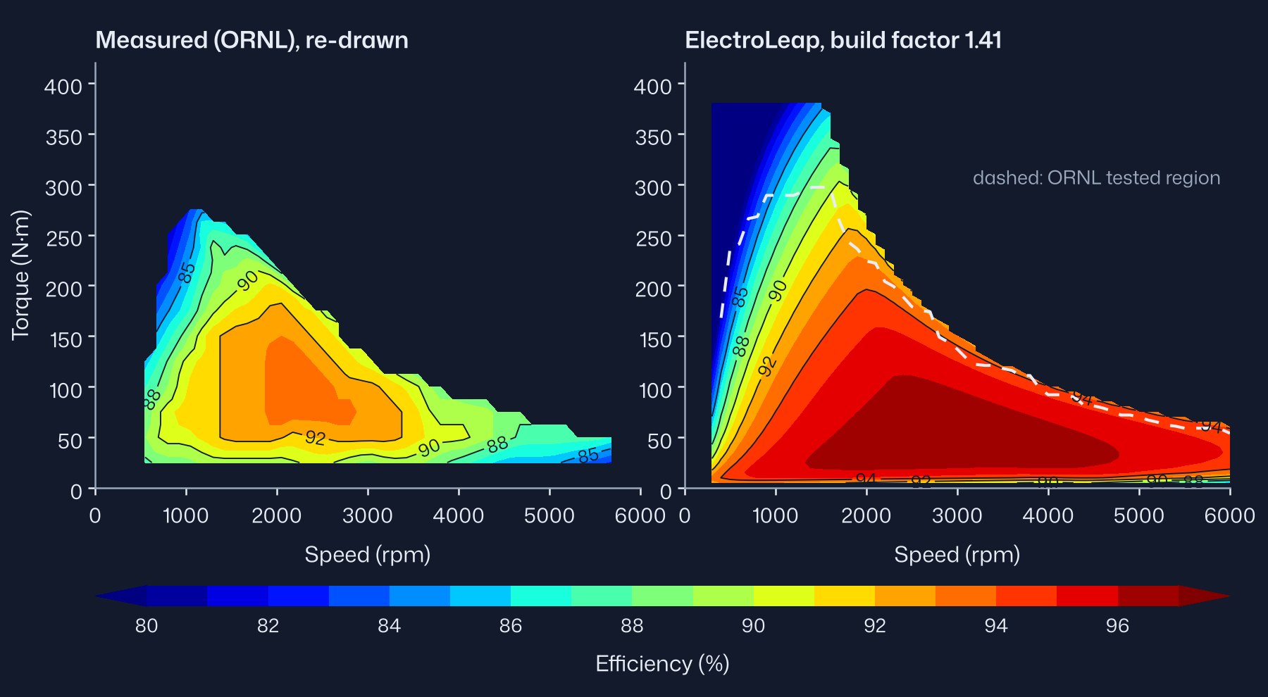
All 94 digitised points lie inside the model's operating envelope. The model is above the measured band at every one of them, by 4.48 % on average without the factor and 4.05 % with it. The direction is the expected one; the size is larger than the 1–2 % we estimated.
| Torque range | Points | Mean excess, no factor (%) | Mean excess, factor 1.41 (%) |
|---|---|---|---|
| Below 50 N·m | 18 | 8.25 | 7.52 |
| 50 to 150 N·m | 55 | 3.97 | 3.56 |
| 150 to 250 N·m | 17 | 2.59 | 2.38 |
| 250 N·m and above | 4 | 2.47 | 2.33 |
| All | 94 | 4.48 | 4.05 |
In watts, the model reproduces about half the measured loss: the mean ratio of model loss to measured loss is 0.49 without the factor and 0.54 with it. The missing loss has two parts. One grows with speed and is consistent with PWM ripple loss in the iron and magnets, and with bearing and oil drag, since the motor ran in oil in its own casing. The other grows with torque at fixed speed, from about 220 W at 25 N·m to 1490 W at 275 N·m at 1000 rpm, and points to copper: the test winding was up to about 100 °C hotter than the model's, and the AC resistance and current ripple under load add to it. The data cannot separate these terms.
The efficiency gap is largest at light load because the missing loss is a larger share of a small output, not because it is largest in watts. For a designer the conclusion is practical: a sinusoidal-current model without mechanical losses gives the electromagnetic part of the loss well, and ripple, AC copper and mechanical losses must be added before its efficiency is compared with an inverter-fed test.
12Torque–speed envelope
The maximum torque at each speed comes from the flux map, with no new field solve, at 500 V dc, winding at 100 °C and magnets at 80 °C. The current behind the 400 N·m rating is not published, so the current limit is the one at which the model reaches 400 N·m: 305.5 A peak with the magnets at 80 °C. For this curve the flux map was extended to 330 A; on the same grid it reproduces the map of §11 within 0.02 N·m at 280.4 A. The voltage limit is 274.2 V phase peak, linear modulation of the 500 V bus, which is the product default.
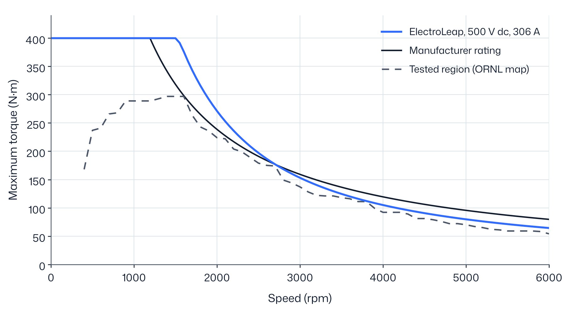
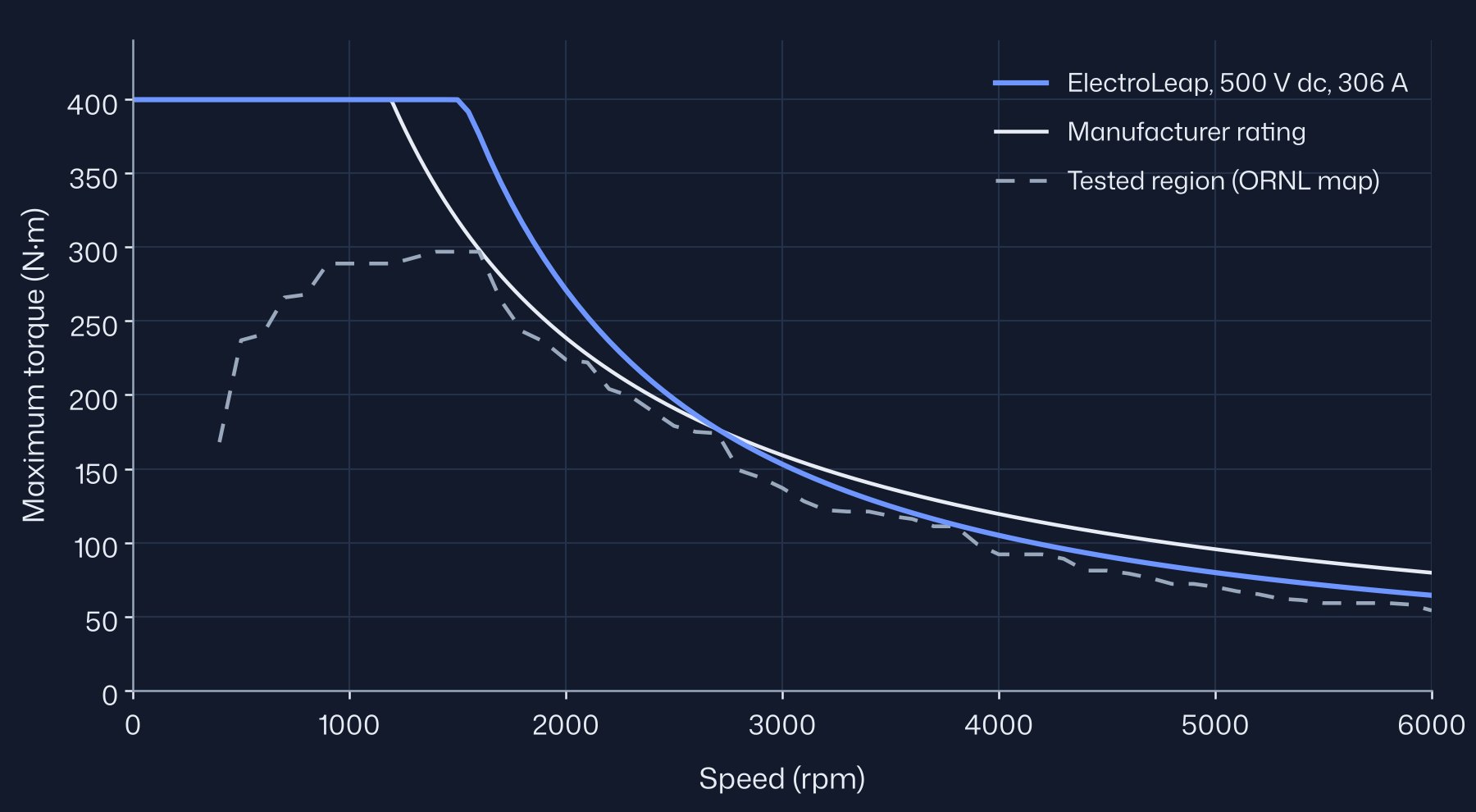
The model holds 400 N·m up to 1500 rpm, above the rated 1200 rpm, and the power peaks at 64 kW near 1550 rpm. It is 57 kW at 2000 rpm and 40 kW at 6000 rpm. The model curve lies above the tested region at every speed. For comparison, the current that gives 400 N·m with the magnets at 25 °C is 280.4 A, the limit used for the efficiency map in §11; ORNL's own estimate, about 325 A, was not measured.
Above about 2700 rpm the curve falls below the 50 kW rating line. The curve uses linear modulation; the Prius inverter over-modulates at high speed, as the test report notes for the efficiency map, and full over-modulation (full-wave operation) gives up to 16 % more voltage, so the model curve is conservative at high speed. The 50 kW rating is a 20-second system rating, not an electromagnetic limit.
13Inductances
The d- and q-axis inductances below are computed with frozen permeability at the current angle of maximum torque per ampere. They were not measured, so they are given for reference only.
| Current (A) | Ld (mH) | Lq (mH) | Lq / Ld | Angle of maximum torque per ampere |
|---|---|---|---|---|
| 150 | 2.031 | 3.774 | 1.86 | 43.2° |
| 250 | 1.812 | 3.065 | 1.69 | 48.3° |
14What the model does not consider at this stage
- Mechanical losses: bearings, windage and oil drag. They are in every measured loss and efficiency.
- PWM ripple: the extra iron, magnet and copper loss from the inverter switching. The model uses sinusoidal currents.
- AC copper loss: skin and proximity effects in the conductors.
- End effects: end-winding leakage and end-region flux. The model is two-dimensional.
- The lamination grade: not published. M270-35A stands in for it, and the voltage sweep in §9 suggests the real steel saturates later.
- Per-point temperatures on the efficiency map: not published. The model uses one winding and one magnet temperature for the whole map.
Each item moves the model in a known direction, and the differences above follow those directions. Adding them is the next step for the loss and efficiency comparisons; the torque and current comparisons do not depend on them.
15Mesh convergence
Mesh convergence was checked on three meshes of the model with the published magnet data, refined throughout, and the converged value estimated by Richardson extrapolation from the three. The default mesh is within 0.07 % of that estimate on every quantity, so every result in this note uses it. With the calibrated magnets, the back-EMF on the 95,380-element mesh differs from the default mesh by 0.05 %.
| Elements over one pole | 26,892 (default) | 95,380 | 359,200 | Extrapolated | Default-mesh error |
|---|---|---|---|---|---|
| Back-EMF constant (V/krpm) | 105.304 | 105.259 | 105.249 | 105.247 | 0.055 % |
| Peak torque at 150 A (N·m) | 252.530 | 252.529 | 252.506 | 252.498 | 0.013 % |
| Peak torque at 250 A (N·m) | 386.693 | 386.940 | 386.948 | 386.948 | 0.066 % |
| Time per position, no load | 2.0 s | 11.8 s | 25.7 s | ||
| Time per position, 150 and 250 A | 2.5 s | 14.1–14.6 s | 57–63 s |
The torque values on the two finer meshes come from a window of positions around the peak; the default-mesh peaks are the full 0–90° sweeps. The 150 A sequence is not monotone, so its estimate uses second order.
16Sources
- [1] T. A. Burress et al., Evaluation of the 2010 Toyota Prius hybrid synergy drive system, ORNL/TM-2010/253, 2011. Used for the 2004 design table and the magnet data.
- [2] J. S. Hsu et al., Report on Toyota/Prius motor design and manufacturing assessment, ORNL/TM-2004/137, 2004. Air-gap flux density, magnet line.
- [3] J. S. Hsu et al., Report on Toyota/Prius motor torque capability, torque property, no-load back EMF and mechanical losses, ORNL/TM-2004/185, revised 2007. Locked-rotor method, back-EMF traces, loss method.
- [4] J. S. Hsu et al., Report on Toyota Prius motor thermal management, ORNL/TM-2005/33, 2005. Lamination drawing, 900 rpm tests.
- [5] R. H. Staunton et al., Evaluation of 2004 Toyota Prius hybrid electric drive system, ORNL/TM-2006/423, 2006. Ratings, locked-rotor and back-EMF tables, no-load loss, efficiency map.
The measured data are from the reports above, published by Oak Ridge National Laboratory for the US Department of Energy. The authors are not affiliated with ElectroLeap and have not reviewed this work. All figures are drawn from the data; the measured curves are digitised from the reports. Toyota and Prius are trademarks of Toyota Motor Corporation; ElectroLeap is not affiliated with or endorsed by Toyota.
Version 1.0, November 2026. Results computed with the ElectroLeap solver as of that date. Corrections or questions: contact us.